2. Composing stimuli, composed stimuli

Most stimuli consist not just of one shape or element, but consist of a composition of multiple components. The geometric components form the basic building blocks for all stimuli implemented in stimupy. In this tutorial, we will explore how a simple example stimulus consisting of multiple geometric elements, can be composed using the functions that generate components.

import numpy as np
import matplotlib.pyplot as plt

from stimupy.utils import plot_stim, plot_stimuli
from stimupy.components import shapes

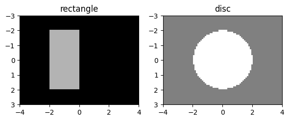
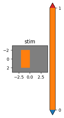
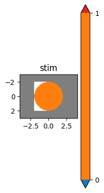
First, we will create the two components that we want to combine in our example; here we will use the rectangle and disc (from our previous tutorial)

rectangle = shapes.rectangle(visual_size=(6,8), ppd=10,
                        rectangle_size=(4,2), rectangle_position=(1,2),
                        intensity_rectangle=.7)

disc = shapes.disc(visual_size=(6,8), ppd=10,
                        radius=2,
                        intensity_disc=1, intensity_background=.5)

plot_stimuli({"rectangle": rectangle, "disc": disc})
plt.show()

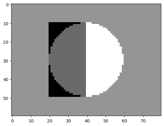
Since the "img"s of the two stimuli are numpy.ndarrays, the simplest manipulation that we can perform to combine our components is to add or subtract them:

new_img = disc["img"] - rectangle["img"]

plt.imshow(new_img, cmap="gray")

<matplotlib.image.AxesImage at 0x7fd57130a110>

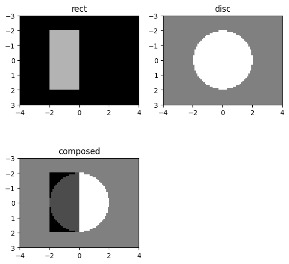
We can even turn this new stimulus-array into something that resembles a stimupy stimulus more – in order to use stimupy tooling like plot_stimuli on it – simply by wrapping it in a dict, and optionally adding some additional metadata:

new_stim = {
  "img": new_img,
  "visual_size": disc["visual_size"],
  "ppd": disc["ppd"]
}

plot_stimuli({"rect": rectangle, "disc": disc, "composed": new_stim})

2.1. Masked regions

The downside of this, is that such an operation (-) on the "img"s uses the whole "img"s, including the background. In other words, these operations aren’t content aware; they treat all pixels the same, rather than restricting operations to the regions that we care about (e.g., the geometric shapes). In many cases, however, we might want to have more control, for instance only subtracting stimulus regions in which the two shapes overlap.

For this, we would like to introduce one key feature of stimupy: stimulus "mask"s. Just like the "img", the stimulus "mask" is a numpy.ndarray which can be found in the stimulus-dict. Each entry of the stimulus "mask" corresponds to a pixel in "img" (i.e., it has the same shape as "img").

Importantly, the "mask" contains only integer-values (compared to the floating point pixel-intensities in "img"). Each integer-value in the mask, corresponds to a geometric region of interest, e.g. the shape. For basic shapes like these there are only two such regions: the background (mask value: 0), and the shape itself (mask value: 1). These can be used to subset or mask the regions: all pixels with value 1 belong to the shape.

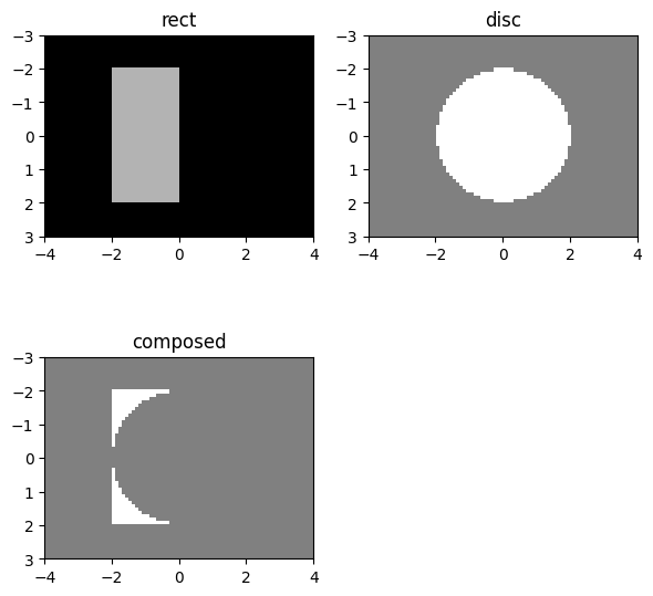
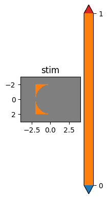
2.2. Composition using masks

We can use these masks to more precisely define how we want to compose our stimulus. Here, we’re removing part of the rectangle where it overlaps with the disc

# Create a new stimulus, i.e., a new dict
composition = {}

# Copy over the two masks
composition["rectangle_mask"] = rectangle["rectangle_mask"]
composition["disc_mask"] = disc["ring_mask"]

# Logically combine masks: rectangle mask, except where ellipse mask:
composition["anti_join_mask"] = (composition["rectangle_mask"] == 1) & (~(composition["disc_mask"]==1))

# Create image:
composition["img"] = np.where(composition["anti_join_mask"], 1, .5)

# Add some metadata
composition["visual_size"] = disc["visual_size"]
composition["ppd"] = disc["ppd"]


plot_stimuli({"rect": rectangle, "disc": disc, "composed": composition})

numpy.where() is a function to create a numpy.ndarray, based on some predicate-array. For each array entry in the predicate (here: the "anti_join_mask"), if it is “truth-y” (True, or nonzero) fill in one value (here: 1); and if the predicate is false, fill in another value (here: .5).

Thus: everywhere the "anti_join_mask" is nonzero: 1; everywhere else: .5

and since each of the masks ("rectangle_", "disc_" and "anti_join_" ) are part of the composition-dict, we can also display each of the different masks:

plt.subplot(1,3,1)
plot_stim(composition, mask="rectangle_mask")
plt.subplot(1,3,2)
plot_stim(composition, mask="disc_mask")
plt.subplot(1,3,3)
plot_stim(composition, mask="anti_join_mask")
plt.show()

2.3. Composed stimuli

This example just highlighted the basics of composition, but this concept underlies a lot of visual stimuli – both in stimupy and in general.

As another example, let’s build a more realistic stimulus – a bullseye: a central disc, surrounded by one or more ring(s).

First, we create our constinuent components:

# Define resolution parameters
visual_size = (10,12)
ppd = 10


# Create center (target) disc:
disc = shapes.disc(visual_size=visual_size, ppd=ppd,
                   radius=2,
                   intensity_disc=.5, intensity_background=.5)

# Create first ring, white:
ring_1 = shapes.ring(visual_size=visual_size, ppd=ppd,
                     radii=(2, 3),
                     intensity_ring=1, intensity_background=.5)

# Create second ring, black:
ring_2 = shapes.ring(visual_size=visual_size, ppd=ppd,
                     radii=(3, 4),
                     intensity_ring=0, intensity_background=.5)

Now we combine the masks into one. We start with the "mask" from the disc, which is 1 for the pixels that are part of the disc and 0 everywhere else. We’ll have to combine this with the "ring_mask"s of each of the rings. These, again, are 1 for the pixels that are part of that ring, and 0 everywhere else. Thus, we take the mask from the disc, and everywhere the first "ring_mask" is True (i.e., not 0) we fill in 2, and everywhere the "ring_mask" is False (i.e., 0) we keep the mask value we already have. Then we repeat this for the second "ring_mask", now filling in the next index 3.

# Accumulate mask, starting with disc mask
mask = disc["ring_mask"]

# Add first ring mask
mask = np.where(ring_1["ring_mask"], 2, mask)

# Add second ring mask
mask = np.where(ring_2["ring_mask"], 3, mask)

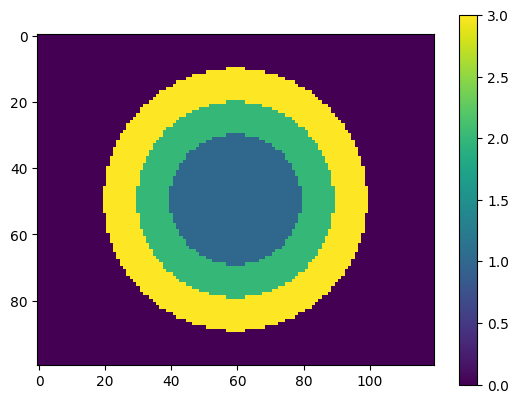
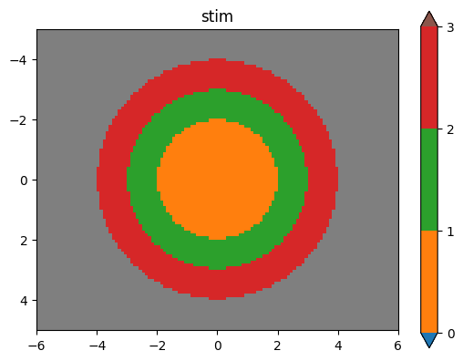
This gives a mask with 4 unique values

np.unique(mask)

array([0, 1, 2, 3])

which each index pixels belonging to different areas:

• 1 for the central disc

• 2 for the first ring around that

• 3 for the outer ring

• 0 for the background, i.e., everywhere else

plt.imshow(mask)
plt.colorbar()

<matplotlib.colorbar.Colorbar at 0x7fd56edbc890>

We can use this mask to now create our new "img", and wrapt everything as stimulus-dict:

# Create a new stimulus, i.e., a new dict
bullseye = {}

# Create the image
bullseye["img"] = np.where(mask==1, 0.5, 0.5)
bullseye["img"] = np.where(mask==2, 1, bullseye["img"])
bullseye["img"] = np.where(mask==3, 0, bullseye["img"])

# Add mask and some metadata
bullseye["mask"] = mask
bullseye["visual_size"] = visual_size
bullseye["ppd"] = ppd

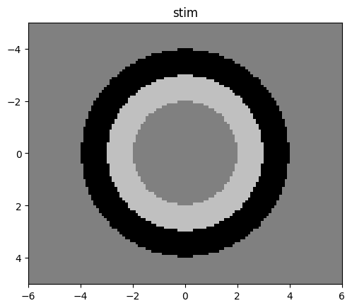
This has created the bullseye stimulus that we want, and included with this is a mask that can separately indicate each of the three regions (and background). We can easily visualize this mask as well, overlaid as colorcoding on top of the stimulus:

plt.subplot(1,2,1)
plot_stim(bullseye)
plt.subplot(1,2,2)
plot_stim(bullseye, mask="mask")
plt.show()

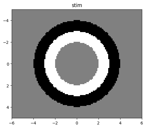
2.4. Using masks to alter the simulus after creation

One advantage of having these kinds of "mask"s that index regions (rather than just binary masks) is that we can use the "mask" to selectively alter one region in an existing stimulus without having to recreate the whole image:

# Change intensity of middle ring to .75; leave rest of image as is:
bullseye["img"] = np.where(bullseye["mask"]==2, .75, bullseye["img"])

plot_stim(bullseye)
plt.show()

2.5. Streamlining with functions

In the above example we had to do some manual operations, primarily

1. Combining the three masks (disc, ring 1 and ring 2) into a single mask

2. Drawing the new stimulus image based on this mask.

Considering that this is a pretty standard workflow, stimupy provides a couple of useful functions to streamline this: stimupy.components.combine_masks(), and stimupy.components.draw_regions():

from stimupy.components import combine_masks, draw_regions

bullseye_mask = combine_masks(disc["ring_mask"], ring_1["ring_mask"], ring_2["ring_mask"])

bullseye_img = draw_regions(mask=bullseye_mask, intensities=[0.5, 1, 0], intensity_background=0.5)

stim = {
  "img": bullseye_img,
  "visual_size": disc["visual_size"]
}

plot_stim(stim)
plt.show()

2.6. Stimuli, components, with multiple regions

Here we have composed a bullseye stimulus from separate components (central disc, inner ring, and outer ring). However, for some such stimuli that consist of a pattern of multiple, consecutive regions, stimupy provides functions to generate directly and does the composition for you.

For the bullseye stimulus, we can use stimupy.components.radials.rings(), which takes in a set of (outer) radii of each ring (and central disc), and an equal number of intensity_rings. These functions generate the full composed stimulus-dict, including the "img", a "mask" with index for each element, and metadata.

from stimupy.components.radials import rings

stim = rings(visual_size=visual_size, ppd=ppd,
             radii=(2, 3, 4),
             intensity_rings=(0.5, 1, 0),
             intensity_background=0.5)

plot_stim(stim, mask="ring_mask")
print(stim.keys())

dict_keys(['edges', 'distance_metric', 'rotation', 'shape', 'visual_size', 'ppd', 'distances', 'origin', 'ring_mask', 'img', 'intensity_rings', 'radii', 'intensity_background'])

2.7. Summary

This tutorial highlights the principle of composition in stimupy. stimupy provides functions to draw several (relatively) simple stimupy.components. These form the basic building blocks from which stimuli with multiple geometric regions or elements can be composed.

The general workflow is to

1. generate the constituent components

2. combine the masks of the components, to produce a mask for the composition

3. use the composed mask to draw the constituent regions of the composed stimulus

stimupy provides some helper-functions to facilitate this. Moreover, there are also some stimupy.components functions for compositions that are repetitions of similar elements:

• stimupy.components.angulars.segments()

• stimupy.components.frames.frames()

• stimupy.components.radials.rings()