1. A first stimulus

Here you will be introduced to the basics of stimupy, and create your first stimulus through this package. At its core, stimupy provides a large number of functions that each draw some kind of (visual) component in a numpy.ndarray.

Tip

Launch on Binder This page can also be launched as an interactive Jupyter Notebook on Binder – see icon at top

1.1. Drawing a basic shape

The most basic stimuli that stimupy provides, are basic geometric shapes. These functions can be found in the stimupy.components.shapes module. To be able to access these, we first have to import this module into our current Python session:

from stimupy.components import shapes

Tip

In some interactive Python interpreters, such as IPython, or Jupyter Notebooks, you can also see all contents of a module by typing the (imported) module name and pressing to autocomplete:

>>> shapes.<TAB>

This module contains the following functions:

Show code cell source Hide code cell source

print(f"Available basic shapes: {shapes.__all__}")

Available basic shapes: ['rectangle', 'triangle', 'cross', 'parallelogram', 'ellipse', 'circle', 'wedge', 'annulus', 'disc', 'ring']

Each of these strings represents a separate function. Let’s take a look at one of them:

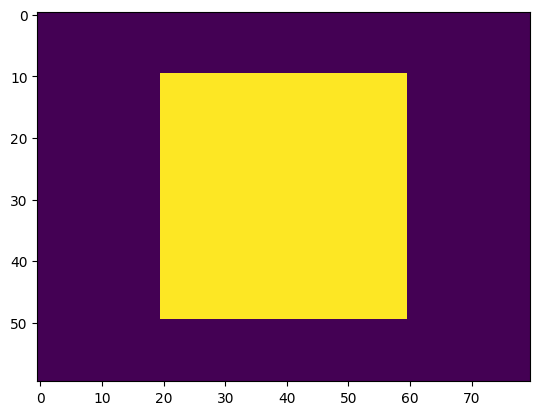
stim = shapes.rectangle(visual_size=(6,8), ppd=10, rectangle_size=(4,4))

This function creates an image, and draws a rectangle inside it. Every pixel which is not part of the rectangle, is considered the “background”. It returns a dictionary, mapping strings as keys, to all kinds of values.

One of these values in in this output dict, is the generated stimulus image is under the key "img". This "img" is a numpy.ndarray, where each entry in this array corresponds to a pixel in the image.

To visualize the stimulus, you can use your preferred way of showing a numpy.ndarray on the stim["img"] array, e.g. matplotlib.pyplot.imshow():

Show code cell source Hide code cell source

import matplotlib.pyplot as plt
plt.imshow(stim["img"])
plt.show()

For convenience, however, stimupy provides a .utils.plot_stim function:

from stimupy.utils import plot_stim

plot_stim(stim)
plt.show()

The values of the entries in the "img" numpy.ndarray represent the pixel intensities, by default in range \([0,1]\).

1.2. Stimulus parameters

All stimupy stimulus-functions require and take multiple arguments. To see what arguments a given function takes, and what each of these arguments controls, you can look at the (online) function reference – or access the function docstring from within Python:

help(shapes.rectangle)

Help on function rectangle in module stimupy.components.shapes:

rectangle(visual_size=None, ppd=None, shape=None, rectangle_size=None, rectangle_position=None, intensity_rectangle=1.0, intensity_background=0.0, rotation=0.0)
    Draw a rectangle
    
    Parameters
    ----------
    visual_size : Sequence[Number, Number], Number, or None (default)
        visual size [height, width] of image, in degrees visual angle
    ppd : Sequence[Number, Number], Number, or None (default)
        pixels per degree [vertical, horizontal]
    shape : Sequence[Number, Number], Number, or None (default)
        shape [height, width] of image, in pixels
    rectangle_size : Number, Sequence[Number, Number]
        rectangle size [height, width], in degrees visual angle
    rectangle_position : Number, Sequence[Number, Number], or None (default)
        position of the rectangle, in degrees visual angle.
        If None, rectangle will be placed in center of image.
    intensity_rectangle : float, optional
        intensity value for rectangle, by default 1.0
    intensity_background : float, optional
        intensity value of background, by default 0.0
    rotation : float, optional
        rotation (in degrees), counterclockwise, by default 0.0 (horizontal)
    
    Returns
    -------
    dict[str, Any]
        dict with the stimulus (key: "img"),
        mask with integer index for the shape (key: "rectangle_mask"),
        and additional keys containing stimulus parameters

The arguments consist of three main categories:

• image size & resolution:

  • visual_size (height, width) of the whole image, in degrees visual angle

  • pixels per degree (ppd) of visual angle

  • shape in pixels

  • because these three are inter-dependent, only two out of 3 need to be specified (see resolution guide for more information)

• component geometry:

  • rectangle_size in degrees visual angle

  • rectangle_position, as distance from top-left corner, in degrees visual angle

• intensity (“photometric”):

  • in this case: intensity_rectangle and intensity_background

  • all stimupy stimuli by default are in the range [0, 1]

For these simple shapes, the arguments should be quite intuitive. To change the geometry of the rectangle, for example make it half its width, we call the function with rectangle_size=(4,2) (changed from (4,4)):

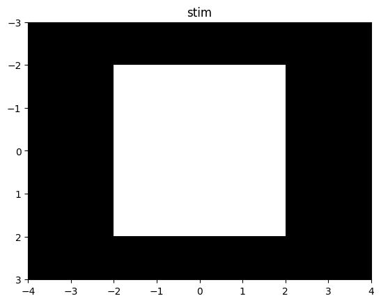
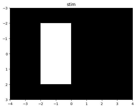
stim = shapes.rectangle(visual_size=(6,8), ppd=10,
                        rectangle_size=(4,2), rectangle_position=(1,2))

plot_stim(stim)
plt.show()

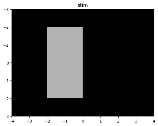
We can also change the intensity of the rectangle that gets drawn:

stim = shapes.rectangle(visual_size=(6,8), ppd=10,
                        rectangle_size=(4,2), rectangle_position=(1,2),
                        intensity_rectangle=.7)

plot_stim(stim)
plt.show()

1.3. Another shape

Let’s look at another example shape – disc:

help(shapes.disc)

Help on function disc in module stimupy.components.radials:

disc(visual_size=None, ppd=None, shape=None, radius=None, intensity_disc=1.0, intensity_background=0.0, origin='mean')
    Draw a central disc
    
    Essentially, `dics(radius)` is an alias for `ring(radii=[0, radius])`
    
    Parameters
    ----------
    visual_size : Sequence[Number, Number], Number, or None (default)
        visual size [height, width] of image, in degrees
    ppd : Sequence[Number, Number], Number, or None (default)
        pixels per degree [vertical, horizontal]
    shape : Sequence[Number, Number], Number, or None (default)
        shape [height, width] of image, in pixels
    radius : Number
        outer radius of disc in degree visual angle
    intensity_disc : Number, optional
        intensity value of disc, by default 1.0
    intensity_background : float, optional
        intensity value of background, by default 0.0
    origin : "corner", "mean" or "center", optional
        if "corner": set origin to upper left corner
        if "mean": set origin to hypothetical image center (default)
        if "center": set origin to real center (closest existing value to mean)
    
    Returns
    -------
    dict[str, Any]
        dict with the stimulus (key: "img"),
        mask with integer index for each ring (key: "ring_mask"),
        and additional keys containing stimulus parameters

Again, this function takes various arguments. The resolution arguments are the same (as they are for all stimupy components and stimul), and the photometric intensity arguments are similar. The component geometry arguments are of course different, specific to the shape that the function provides.

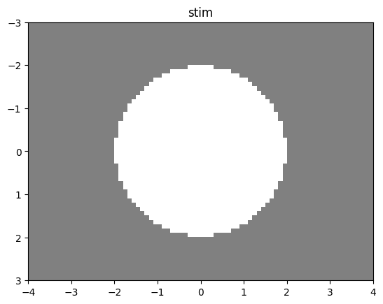
disc = shapes.disc(visual_size=(6,8), ppd=10,
                        radius=2,
                        intensity_disc=1, intensity_background=.5)

plot_stim(disc)
plt.show()

1.4. Stimulus parameters are part of output

When we take a closer look at the whole output dictionary, we see that all of the input parameters to the function are also there:

print(stim)

As you can see, this output also contains all of the parameters for the component, both those that we specified (e.g., visual_size, intensity_rectangle), but also those for which default values were used (e.g., intensity_background). Thus, this output is self-documenting: all the necessary information to produce this stimulus are in the stimulus-dict.

A nice feature of these dicts is that you, the user, can add any arbitrary (meta)data to them, after creating the stimulus. For instance, we can add some label, or a creation date:

stim["label"] = "A nice stimulus"
stim["date"] = "today"

print(stim)

{'img': array([[0., 0., 0., ..., 0., 0., 0.],
       [0., 0., 0., ..., 0., 0., 0.],
       [0., 0., 0., ..., 0., 0., 0.],
       ...,
       [0., 0., 0., ..., 0., 0., 0.],
       [0., 0., 0., ..., 0., 0., 0.],
       [0., 0., 0., ..., 0., 0., 0.]]), 'rectangle_mask': array([[0, 0, 0, ..., 0, 0, 0],
       [0, 0, 0, ..., 0, 0, 0],
       [0, 0, 0, ..., 0, 0, 0],
       ...,
       [0, 0, 0, ..., 0, 0, 0],
       [0, 0, 0, ..., 0, 0, 0],
       [0, 0, 0, ..., 0, 0, 0]]), 'visual_size': Visual_size(height=6.0, width=8.0), 'ppd': Ppd(vertical=10.0, horizontal=10.0), 'shape': Shape(height=60, width=80), 'rectangle_size': Visual_size(height=4.0, width=2.0), 'rectangle_position': array([1, 2]), 'intensity_background': 0.0, 'intensity_rectangle': 0.7, 'rotation': 0.0, 'label': 'A nice stimulus', 'date': 'today'}

1.5. Summary

This tutorial highlights the core design principles of stimupy-stimuli. At its simplest, a stimupy-stimulus is:

1. a plain Python dict,

2. containing a numpy.ndarray as the "img" key.

3. (produced by a stimulus or component function)

The advantages of this are:

1. the actual image can easily be integrated in existing codebases:

   • save to file using numpy.save(), matplotlib.pyplot.imsave(), or PIL

   • manipulate using any numpy-based code

2. anything that is compliant with this basic structure can use (some of) stimupy tooling, e.g., plot_stim, exports, or contrast manipulations to name a few

3. since Python dicts are mutable, you as user can add, create, remove, rename any of the keys and values.

The main disadvantage is that there are no controls or guarantees after a stimulus is created for the accuracy of any of its fields, since the user can manually change values at any point in time.