Axes, orientations, and distance metrics#
Digital images have a natural coordinate scheme with two axes: a vertical \(y\)-axis, and horizontal \(x\)-axis.
This is how pixels are organized in a screen,
and this is how the pixel-intensities are encoded as image matrices (e.g., numpy.ndarray).
But not all stimuli are most sensible defined in these coordinates,
and stimupy has several more axes and distances it can use.
Horizontal, vertical, oblique#
As mentioned, all images have a natural vertical and horizontal axes.
Where used, stimupy expects them in this order: (y, x) or (height, width)
– in line with computer science and specifically NumPy conventions.
Thus visual_size=(12, 16) indicates and image
that is \(12\) degrees high, and \(16\) degrees wide.
Positions, too, are generally specified in these coordinates:
rectangle_position=(2, 1) places the rectangle
\(3\) degrees from the top and \(5\) degree to the right:
from stimupy.components import shapes
from stimupy.utils import plot_stim

stim = shapes.rectangle(visual_size=(12, 16), ppd=10,
                        rectangle_size=(4, 4),
                        rectangle_position=(3, 5))

plot_stim(stim)
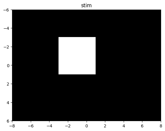
<Axes: title={'center': 'stim'}>
While the image-axes are vertical & horizontal,
stimupy allows you to easily draw oblique or rotated stimuli.
Almost all stimulus-functions have a rotation argument,
which expresses the rotation in degrees, from counterclockwise from the 3 o’clock position
(in line with angles around a unit circle).
Note that the stimulus size is determined along the rotated \(y, x\) axes,
but the image size and stimulus position are in the original frame of reference.
stim = shapes.rectangle(visual_size=(12, 16), ppd=10,
                        rectangle_size=(4, 4),
                        rectangle_position=(3, 5),
                        rotation=30)

plot_stim(stim)
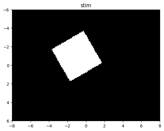
<Axes: title={'center': 'stim'}>
Radial#
Some stimuli are more naturally defined not along a linear axis like the horizontal, vertical, and rotated/oblique axes. One example of this is a circle, which is more naturally defined using a given radius, radiating outwards from a point of origin.
stim = shapes.circle(visual_size=(12, 16), ppd=10,
                     radius=2)

plot_stim(stim)
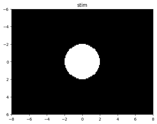
<Axes: title={'center': 'stim'}>
Here the point of origin is by default the center of the image,
but this can be changed
The origin parameter can be an actual center pixel,
the hypothetical image mean (if there is no single pixel at this exact location),
or the topleft corner of the image.
stim = shapes.circle(visual_size=(12, 16), ppd=10,
                     radius=2,
                     origin='corner')

plot_stim(stim)
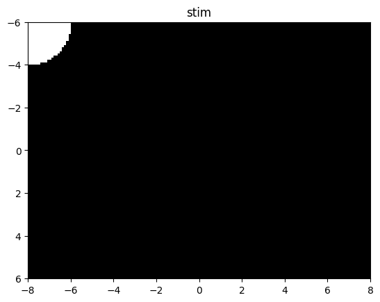
<Axes: title={'center': 'stim'}>
Distance metric#
We term these aforementioned axes a distance_metric,
as they measure distance from some point of origin.
This way of thinking is especially important
for wave specifications in stimupy.components.waves
and their use in wave-like stimuli in stimupy.stimuli.waves.
For the linear metrics (horizontal, vertical, oblique),
those waves measure distance along that axis (from the center by default):
from stimupy.components import waves

stim = waves.sine(visual_size=(12, 16), ppd=10,
                  distance_metric="horizontal",
                  frequency=.2)

plot_stim(stim)
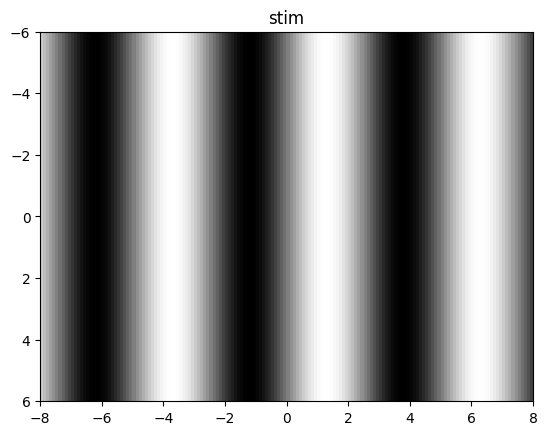
<Axes: title={'center': 'stim'}>
But this can be changed to another origin as well:
stim = waves.sine(visual_size=(12, 16), ppd=10,
                  distance_metric="horizontal",
                  frequency=.2,
                  origin='corner')

plot_stim(stim)
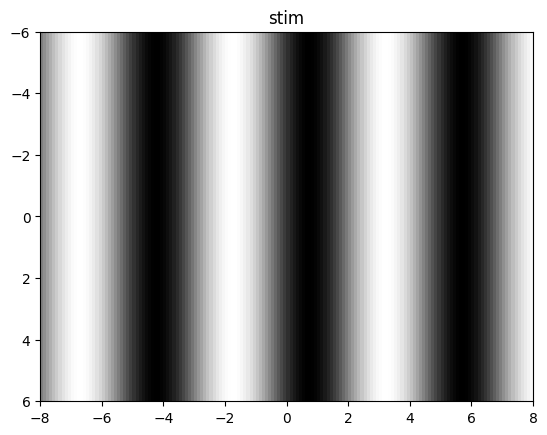
<Axes: title={'center': 'stim'}>
The radial stimuli are a good way of understanding the distance_metric:
each pixel is some distance away from the origin (center by default),
which is the relevant metric for determining whether that pixel
is part of the targeted region:
stim = waves.sine(visual_size=(12, 16), ppd=10,
                  distance_metric="radial",
                  frequency=.2)

plot_stim(stim)
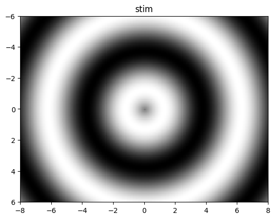
<Axes: title={'center': 'stim'}>
Note
The radial distance is calculated as \(r = \sqrt{x^2 + y^2}\).
Rectilinear#
A more intriguing distance_metric is the rectilinear metric,
which does not correspond to some singular linear axis in the image.
Note
The rectilinear distance is calculated as \(d = \max{x^2, y^2}\)
This creates a frame-like, or “squared-off” radial, distance:
the rectilinear distance of a pixel to the origin
is determined by the largest of the two linear distances.
stim = waves.sine(visual_size=(12, 16), ppd=10,
                  distance_metric="rectilinear",
                  frequency=.2)

plot_stim(stim)
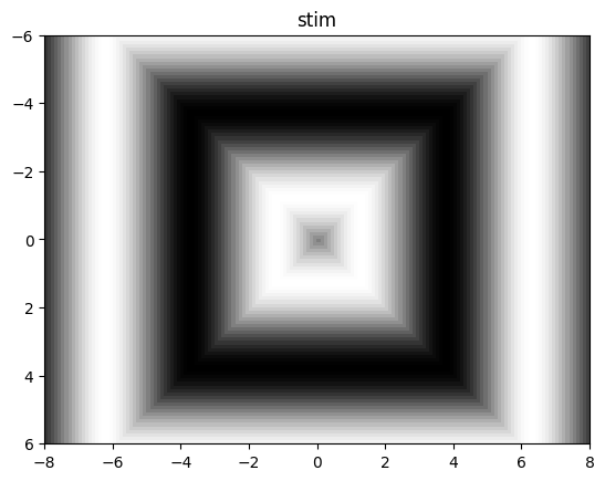
<Axes: title={'center': 'stim'}>
It is related to metrics that are often called “Manhattan”, “taxicab”, “cityblock”.
Angular#
Another interesting distance_metric is the angular distance,
which uniquely has a fixed range of \([0, 360]\).
Note
The angular distance is calculated as the angle from 3 o’clock position (in degrees).
stim = waves.sine(visual_size=(12, 16), ppd=10,
                  distance_metric="angular",
                  frequency=10)

plot_stim(stim)
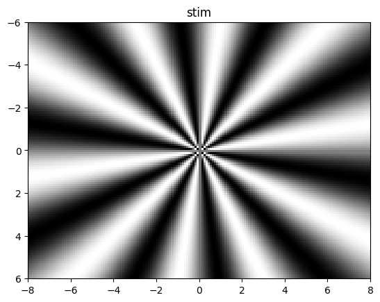
<Axes: title={'center': 'stim'}>