3. Exploring parameterized stimuli

The geometric components are the basic building blocks which can be composed into all kinds of stimuli.

import matplotlib.pyplot as plt
from stimupy.utils import plot_stim

Included in stimupy is a large set of functions to generate known stimuli (see How stimupy is organized) These are generally subdivided into submodules bearing their usual name.

The submodule names are pluralized, so a bullseye stimulus function can be found in stimupy.stimuli.bullseyes.bullseye()

All of these can be accessed by import stimupy.stimuli.<submodule> or from stimupy.stimuli import <submodule>

3.1. Thin wrapper around component - Simultaneous Brightness Contrast (SBC)

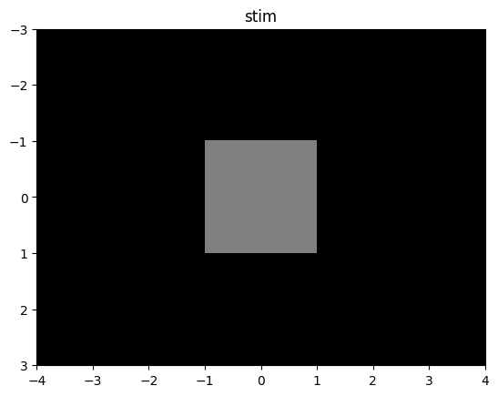
Firstly, a geometrically simple stimulus: a classic Simultaneous Brightness Contrast (SBC) display:

from stimupy.stimuli import sbcs

stim = sbcs.basic(visual_size=(6,8), ppd=10,
                  target_size=(2,2))

plot_stim(stim)
plt.show()

As you can see, this is not (much) more than:

from stimupy.components import shapes

component = shapes.rectangle(visual_size=(6,8), ppd=10,
                             rectangle_size=(2,2),
                             intensity_background=0.0, intensity_rectangle=0.5)

plot_stim(component)
plt.show()

stimuli, like components, also have 3 overall categories of parameters:

• image size & resolution

• stimulus geometry

• stimulus photometry (intensities)

However, some of the stimulus parameters have different names in stimuli. In particular, many stimuli have the concept of a target region(s): image regions that are of some particular scientific interest in this stimulus. For an SBC stimulus, this would be the rectangle. Thus, the sbcs.basic function takes a

• target_size, compared to rectangle_size

• intensity_target, rather than an intensity_rectangle (with a default intermediate value of 0.5)

• In addition, the output stimulus contains a target_mask, which masks the pixels of the target region.

For this specific stimulus, the sbcs.basic provides little use over the base component. But, realistically, we would not show just this one part of a SBC display, but rather show both sides of the SBC displays as implemented in two_sided:

two_sided_stim = sbcs.basic_two_sided(visual_size=(6,8), ppd=10,
                                target_size=(2,2))

plot_stim(two_sided_stim)
plt.show()

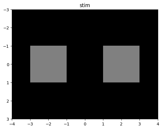
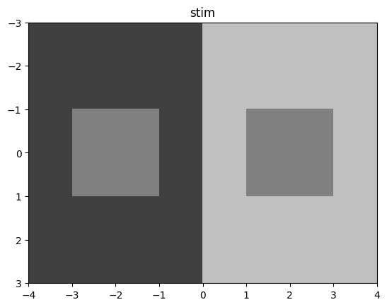
Now we have a true SBC display: two separate image regions, with different background intensities, and physically identical patches embedded in these regions.

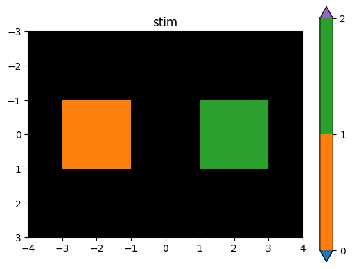
Both patches are part of the same target_mask, although with different integer-indices:

plot_stim(two_sided_stim, mask='target_mask')
plt.show()

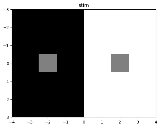
and they are controlled by the same target_size argument:

two_sided_stim = sbcs.basic_two_sided(visual_size=(6,8), ppd=10,
                                target_size=(1,1),
                                intensity_background=(0.0,1.0))

plot_stim(two_sided_stim)
plt.show()

The intensity_background can also be varied at creation:

two_sided_stim = sbcs.basic_two_sided(visual_size=(6,8), ppd=10,
                                target_size=(2,2),
                                intensity_background=(.25,.75))

plot_stim(two_sided_stim)
plt.show()

This stimulus-function provides a significant useful shorthand over manually composing such a display from components, by keeping some parameters consistent between the parts. For this specific function, the two target regions will have the same size and central positioning.

3.2. Parameterized composition - Bullseye

In the previous tutorial we constructed a bullseye stimulus: a central (target) disc, surrounded by one or more rings.

This, too, is a stimulus included in stimupy.stimuli:

from stimupy import bullseyes

stim_bull = bullseyes.circular(
   visual_size=(10,10),
   ppd=10,
   n_rings=5,
   ring_width=1,
)

plot_stim(stim_bull)
plt.show()

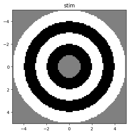
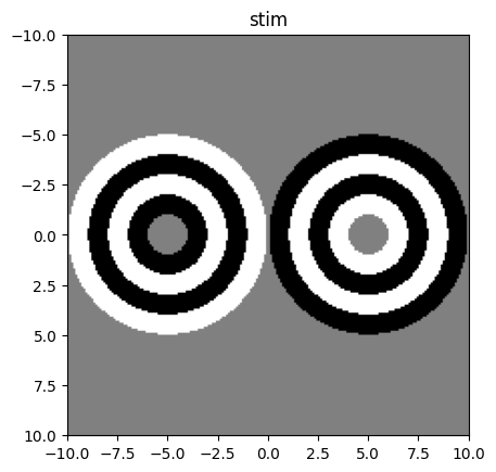
This function provides some higher-level parameterization(s) than our manual composition; we simply specify the number of surrounding rings we want, and the width for each of these. There is also a two-sided display of this stimulus:

stim_2bull = bullseyes.circular_two_sided(
   visual_size=(20,20),
   ppd=10,
   n_rings=5,
   ring_width=1,
  intensity_rings=((0, 1), (1, 0))
)

plot_stim(stim_2bull)
plt.show()

3.3. Multiple paramaterizations - Todorovic illusion

So far, we’ve highlighted some stimuli for which it is quite clear how one would compose them. Generally, though, there can be multiple ways to compose a stimulus and this can have implications for how one would parameterize the composed stimulus.

A good example of this is the Todorovic Illusion, which one can interpret as having a rectangular target that is partially occluded by some “covers” OR as having a cross-shaped target with adjoining squares. For a single stimulus parameterization, these two conceptions may produce perfectly identical images (see fig, top). However, when changing parameters, you would expect different behavior from the stimulus function dependent on your conception/interpretation of the stimulus (see fig, bottom).

from stimupy.stimuli import todorovics
from stimupy.utils import plot_stimuli

resolution = {"visual_size": 5, "ppd": 10}

stims = {
    "cross, covers_size=1" : todorovics.cross(**resolution,     cross_size=2,  cross_thickness=1, covers_size=1),
    "rect, covers_size=1"  : todorovics.rectangle(**resolution, target_size=2, covers_offset=1,   covers_size=1),
    "cross, covers_size=.5": todorovics.cross(**resolution,     cross_size=2,  cross_thickness=1, covers_size=0.5),
    "rect, covers_size=.5" : todorovics.rectangle(**resolution, target_size=2, covers_offset=1,   covers_size=0.5),
}

plot_stimuli(stims)

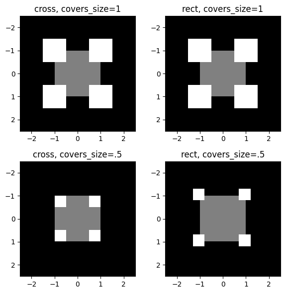
Fig. 3.1 todorovics.cross() (left) and .rectangle() (right) can produce identical images (top) for some parameterizations, but have different behavior for others (bottom)