Create color stimuli

By default, stimupy creates grayscale stimuli with intensity values between 0 and 1. stimupy is primarily focused on stimulus geometry - the shapes, patterns, and spatial arrangements that define visual stimuli. While you can create color stimuli by specifying RGB values directly, proper color specification is a complex topic involving color spaces, calibration, and perceptual considerations that are better handled by specialized color science libraries.

This guide shows you basic approaches to adding color to stimupy stimuli, but for rigorous color work, consider using dedicated color libraries like colorspacious, colour-science, or colorspace.

import numpy as np
import matplotlib.pyplot as plt
from stimupy.components import shapes
from stimupy.stimuli import checkerboards
from stimupy.utils import plot_stim

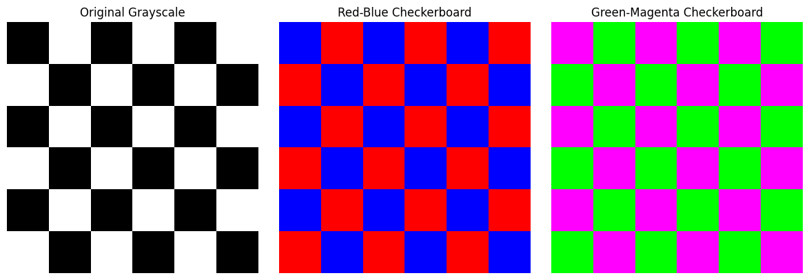
Method 1: Create RGB arrays directly

When to use: When you need basic color specification with known RGB values.

Steps:

1. Create your grayscale stimulus

2. Convert to RGB by expanding dimensions

3. Assign specific RGB color values to different regions

# Step 1: Create base stimulus
checkerboard = checkerboards.checkerboard(visual_size=(6, 6), ppd=20, 
                                         check_visual_size=1, 
                                         intensity_checks=(0, 1))

# Step 2: Create RGB version
height, width = checkerboard["img"].shape
rgb_img = np.zeros((height, width, 3))

# Step 3: Assign colors based on checkerboard pattern
# White squares -> Red
# Black squares -> Blue
mask = checkerboard["img"] > 0.5
rgb_img[mask] = [1, 0, 0]      # Red for white squares
rgb_img[~mask] = [0, 0, 1]     # Blue for black squares

# Display
plt.figure(figsize=(12, 4))
plt.subplot(1, 3, 1)
plt.imshow(checkerboard["img"], cmap="gray")
plt.title("Original Grayscale")
plt.axis('off')

plt.subplot(1, 3, 2)
plt.imshow(rgb_img)
plt.title("Red-Blue Checkerboard")
plt.axis('off')

plt.subplot(1, 3, 3)
# Alternative: Green-Magenta
rgb_img2 = np.zeros((height, width, 3))
rgb_img2[mask] = [0, 1, 0]     # Green
rgb_img2[~mask] = [1, 0, 1]    # Magenta
plt.imshow(rgb_img2)
plt.title("Green-Magenta Checkerboard")
plt.axis('off')

plt.tight_layout()
plt.show()

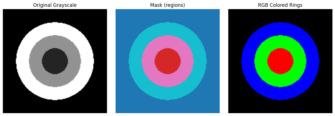
Method 2: Use masks for multi-color stimuli

When to use: When you have complex stimuli with multiple regions that need different colors.

Steps:

1. Create stimulus with mask

2. Create RGB array

3. Use mask to assign different colors to each region

# Step 1: Create stimulus with multiple regions
from stimupy.components.radials import rings

ring_stim = rings(visual_size=(8, 8), ppd=20,
                  radii=(1, 2, 3),
                  intensity_rings=(0.2, 0.5, 0.8),
                  intensity_background=0.1)

# Step 2: Create RGB array
height, width = ring_stim["img"].shape
rgb_rings = np.zeros((height, width, 3))

# Step 3: Assign different colors to each ring
mask = ring_stim["ring_mask"]

# Background (mask == 0) -> Black
rgb_rings[mask == 0] = [0, 0, 0]
# Ring 1 (mask == 1) -> Red
rgb_rings[mask == 1] = [1, 0, 0]
# Ring 2 (mask == 2) -> Green  
rgb_rings[mask == 2] = [0, 1, 0]
# Ring 3 (mask == 3) -> Blue
rgb_rings[mask == 3] = [0, 0, 1]

# Display
plt.figure(figsize=(12, 4))
plt.subplot(1, 3, 1)
plt.imshow(ring_stim["img"], cmap="gray")
plt.title("Original Grayscale")
plt.axis('off')

plt.subplot(1, 3, 2)
plt.imshow(ring_stim["ring_mask"], cmap="tab10")
plt.title("Mask (regions)")
plt.axis('off')

plt.subplot(1, 3, 3)
plt.imshow(rgb_rings)
plt.title("RGB Colored Rings")
plt.axis('off')

plt.tight_layout()
plt.show()

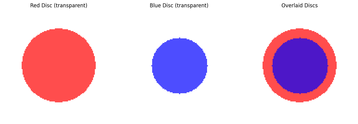
Method 3: Color stimuli with transparency

When to use: When you need to overlay colored stimuli or create transparent effects.

Steps:

1. Create RGBA array (Red, Green, Blue, Alpha)

2. Set alpha channel based on stimulus properties

3. Use for overlays or transparent effects

# Step 1: Create base stimuli
disc1 = shapes.disc(visual_size=(6, 6), ppd=20, radius=2, 
                    intensity_disc=1, intensity_background=0)

disc2 = shapes.disc(visual_size=(6, 6), ppd=20, radius=1.5, 
                    intensity_disc=1, intensity_background=0,
                    origin="center")

# Step 2: Create RGBA arrays
rgba1 = np.zeros((*disc1["img"].shape, 4))
rgba2 = np.zeros((*disc2["img"].shape, 4))

# Red disc with transparency
mask1 = disc1["ring_mask"] == 1
rgba1[mask1] = [1, 0, 0, 0.7]  # Semi-transparent red

# Blue disc with transparency  
mask2 = disc2["ring_mask"] == 1
rgba2[mask2] = [0, 0, 1, 0.7]  # Semi-transparent blue

# Step 3: Display overlays
plt.figure(figsize=(12, 4))

plt.subplot(1, 3, 1)
plt.imshow(rgba1)
plt.title("Red Disc (transparent)")
plt.axis('off')

plt.subplot(1, 3, 2)
plt.imshow(rgba2)
plt.title("Blue Disc (transparent)")
plt.axis('off')

plt.subplot(1, 3, 3)
# Overlay both discs
plt.imshow(rgba1)
plt.imshow(rgba2)
plt.title("Overlaid Discs")
plt.axis('off')

plt.tight_layout()
plt.show()

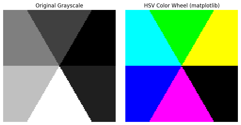
Method 4: Using color space conversions

When to use: When you need to work with specific color spaces or chromaticity coordinates.

Important: This example uses matplotlib’s HSV implementation, but for rigorous color science work, use dedicated libraries like colorspacious, colour-science, or colorspace that provide proper chromaticity-to-RGB conversions, color space transformations, and color appearance models.

Steps:

1. Create stimulus geometry

2. Use a color library to convert from desired color space to RGB

3. Apply the RGB values to your stimulus

from matplotlib.colors import hsv_to_rgb

# Step 1: Create angular segments with different hues
from stimupy.components.angulars import segments

segment_stim = segments(visual_size=(6, 6), ppd=20,
                       angles=(0, 60, 120, 180, 240, 300, 360),
                       intensity_segments=(0.2, 0.4, 0.6, 0.8, 1.0, 0.3),
                       intensity_background=0.1)

# Step 2: Create HSV array (basic matplotlib conversion)
height, width = segment_stim["img"].shape
hsv_img = np.zeros((height, width, 3))

# Assign different hues to each segment
mask = segment_stim["segment_mask"]
for i in range(1, 7):  # 6 segments
    segment_mask = mask == i
    hue = (i - 1) / 6  # Hue from 0 to 1
    hsv_img[segment_mask] = [hue, 1, 1]  # Full saturation and brightness

# Step 3: Convert to RGB using matplotlib (basic conversion)
rgb_img = hsv_to_rgb(hsv_img)

# Display
plt.figure(figsize=(8, 4))
plt.subplot(1, 2, 1)
plt.imshow(segment_stim["img"], cmap="gray")
plt.title("Original Grayscale")
plt.axis('off')

plt.subplot(1, 2, 2)
plt.imshow(rgb_img)
plt.title("HSV Color Wheel (matplotlib)")
plt.axis('off')

plt.tight_layout()
plt.show()

Specifying chromaticities

Note

stimupy focuses on geometry, not color science.

Workflow for specifying chromaticies of stimupy stimuli:

1. Geometry specification: Use stimupy to create the geometric stimulus structure

2. Chromaticity specification: Determine chromaticity coordinates (xy, Lab, etc.) that you want the stimulus/different regions to have

3. Convert to RGB using dedicated color science libraries

   • e.g., colorspacious, colour-science, or colorspace for proper color space conversions

   • Monitor calibration: The conversion of RGB <-> chromaticity is different for different monitors, depends heavily on monitor calibration and viewing conditions

4. Apply RGB values to the stimulus using the methods above

5. Validate colors with calibrated equipment

Color specification reference

Basic RGB values (for display on typical monitors):

• Red: [1, 0, 0]

• Green: [0, 1, 0]

• Blue: [0, 0, 1]

• Yellow: [1, 1, 0]

• Cyan: [0, 1, 1]

• Magenta: [1, 0, 1]

• White: [1, 1, 1]

• Black: [0, 0, 0]

RGBA values: Same as RGB plus alpha (transparency)

• Semi-transparent red: [1, 0, 0, 0.5]

Choosing the right method

Method	Best for	Pros	Cons
RGB arrays	Basic color specification	Simple, direct control	No color science validation
Mask-based	Multi-region stimuli	Clean separation, reusable	Requires planning
RGBA/transparency	Overlays, complex compositions	Advanced effects	More complex
Color space conversion	Scientific color work	Proper color science	Requires additional libraries

For experimental work: Combine stimupy for geometry with dedicated color science libraries for proper chromaticity specification.