Masks

One key feature of stimupy is stimulus "mask"s. Just like the "img", the stimulus "mask" is a numpy.ndarray which can be found in the stimulus-dict. Each entry of the stimulus "mask" corresponds to a pixel in "img" (i.e., it has the same shape as "img").

import numpy as np
import matplotlib.pyplot as plt

from stimupy.utils import plot_stim, plot_stimuli
from stimupy.components import shapes

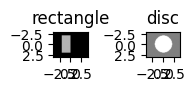
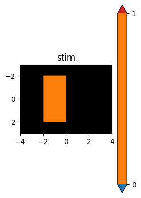
Let’s create a simple example to understand masks:

rectangle = shapes.rectangle(visual_size=(6,8), ppd=10,
                        rectangle_size=(4,2), rectangle_position=(1,2),
                        intensity_rectangle=.7)

disc = shapes.disc(visual_size=(6,8), ppd=10,
                        radius=2,
                        intensity_disc=1, intensity_background=.5)

plot_stimuli({"rectangle": rectangle, "disc": disc})
plt.show()

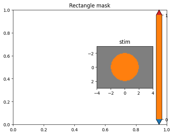
Basic masks

Importantly, the "mask" contains only integer-values (compared to the floating point pixel-intensities in "img"). Each integer-value in the mask, corresponds to a geometric region of interest, e.g. the shape. For basic shapes like these there are only two such regions: the background (mask value: 0), and the shape itself (mask value: 1). These can be used to subset or mask the regions: all pixels with value 1 belong to the shape.

# Display the masks for our shapes
plt.subplot(1,2,1)
plot_stim(rectangle, mask="rectangle_mask")
plt.title("Rectangle mask")
plt.subplot(1,2,2)
plot_stim(disc, mask="ring_mask")
plt.title("Disc mask")
plt.tight_layout()
plt.show()

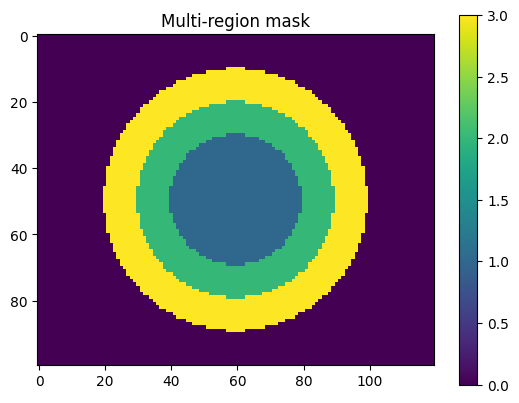
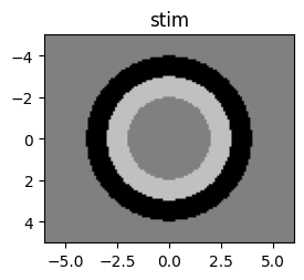
Multi-region masks

Masks can also contain multiple regions, each with different integer values. Let’s create a bullseye with multiple rings to demonstrate this:

# Define resolution parameters
visual_size = (10,12)
ppd = 10

# Create center (target) disc:
disc = shapes.disc(visual_size=visual_size, ppd=ppd,
                   radius=2,
                   intensity_disc=.5, intensity_background=.5)

# Create first ring, white:
ring_1 = shapes.ring(visual_size=visual_size, ppd=ppd,
                     radii=(2, 3),
                     intensity_ring=1, intensity_background=.5)

# Create second ring, black:
ring_2 = shapes.ring(visual_size=visual_size, ppd=ppd,
                     radii=(3, 4),
                     intensity_ring=0, intensity_background=.5)

We can combine multiple masks into one that indexes different regions:

# Accumulate mask, starting with disc mask
mask = disc["ring_mask"]

# Add first ring mask
mask = np.where(ring_1["ring_mask"], 2, mask)

# Add second ring mask
mask = np.where(ring_2["ring_mask"], 3, mask)

print("Unique mask values:", np.unique(mask))

Unique mask values: [0 1 2 3]

This gives a mask with 4 unique values which each index pixels belonging to different areas:

• 1 for the central disc

• 2 for the first ring around that

• 3 for the outer ring

• 0 for the background, i.e., everywhere else

plt.imshow(mask)
plt.colorbar()
plt.title("Multi-region mask")
plt.show()

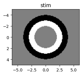
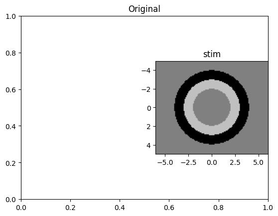
Using masks to manipulate stimuli

One advantage of having these kinds of "mask"s that index regions (rather than just binary masks) is that we can use the "mask" to selectively alter one region in an existing stimulus without having to recreate the whole image:

# Create image using the mask
img = np.where(mask==1, 0.5, 0.5)  # Central disc
img = np.where(mask==2, 1, img)    # First ring
img = np.where(mask==3, 0, img)    # Second ring

bullseye = {
    "img": img,
    "mask": mask,
    "visual_size": visual_size,
    "ppd": ppd
}

plt.subplot(1,2,1)
plot_stim(bullseye)
plt.title("Original")

# Change intensity of middle ring to .75; leave rest of image as is:
bullseye["img"] = np.where(bullseye["mask"]==2, .75, bullseye["img"])

plt.subplot(1,2,2)
plot_stim(bullseye)
plt.title("Modified middle ring")
plt.tight_layout()
plt.show()

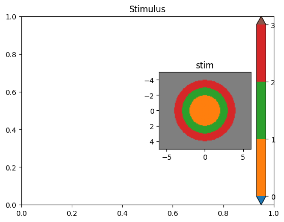
Visualizing masks

We can easily visualize masks overlaid as color coding on top of the stimulus:

plt.subplot(1,2,1)
plot_stim(bullseye)
plt.title("Stimulus")
plt.subplot(1,2,2)
plot_stim(bullseye, mask="mask")
plt.title("With mask overlay")
plt.tight_layout()
plt.show()

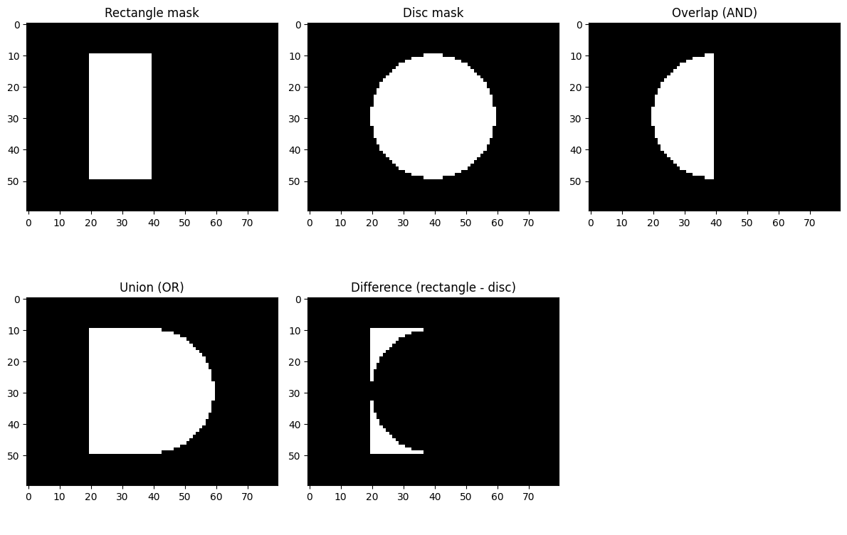
Logical operations on masks

Masks can be combined using logical operations. For example, we can create masks for overlapping regions:

# Create overlapping shapes
rectangle = shapes.rectangle(visual_size=(6,8), ppd=10,
                        rectangle_size=(4,2), rectangle_position=(1,2),
                        intensity_rectangle=.7)

disc = shapes.disc(visual_size=(6,8), ppd=10,
                        radius=2,
                        intensity_disc=1, intensity_background=.5)

# Logical operations on masks
overlap_mask = (rectangle["rectangle_mask"] == 1) & (disc["ring_mask"] == 1)
union_mask = (rectangle["rectangle_mask"] == 1) | (disc["ring_mask"] == 1)
difference_mask = (rectangle["rectangle_mask"] == 1) & (~(disc["ring_mask"] == 1))

# Visualize the different logical operations
fig, axes = plt.subplots(2, 3, figsize=(12, 8))

axes[0,0].imshow(rectangle["rectangle_mask"], cmap="gray")
axes[0,0].set_title("Rectangle mask")
axes[0,1].imshow(disc["ring_mask"], cmap="gray")
axes[0,1].set_title("Disc mask")
axes[0,2].imshow(overlap_mask, cmap="gray")
axes[0,2].set_title("Overlap (AND)")

axes[1,0].imshow(union_mask, cmap="gray")
axes[1,0].set_title("Union (OR)")
axes[1,1].imshow(difference_mask, cmap="gray")
axes[1,1].set_title("Difference (rectangle - disc)")
axes[1,2].axis('off')

plt.tight_layout()
plt.show()

numpy.where() is a function to create a numpy.ndarray, based on some predicate-array. For each array entry in the predicate (here: a mask), if it is “truth-y” (True, or nonzero) fill in one value; and if the predicate is false, fill in another value.

Masks are fundamental to how stimupy works and enable precise control over different regions of stimuli, making it easy to create complex visual patterns and manipulate them after creation.