Compose stimuli from components

Most visual stimuli consist of multiple geometric elements combined together. For example, a Gabor is a composition of a sinusoidal grating and a Gaussian envelope.

Note

Many common stimulus compositions are already implemented in stimupy.stimuli (checkerboards, Gabors, plaids, etc.). The methods in this guide are primarily for when you need to create custom compositions that aren’t available as pre-built functions.

This guide shows you different ways to compose stimuli from the basic geometric components that stimupy provides.

import numpy as np
import matplotlib.pyplot as plt

from stimupy.utils import plot_stim, plot_stimuli
from stimupy.components import shapes

Method 1: Direct composition functions

When to use: For common patterns where stimupy provides dedicated functions. Start here - check if your desired composition already exists before building from scratch.

Available types:

• Geometric patterns: stimupy.components.radials.rings(), stimupy.components.angulars.segments(), stimupy.components.frames.frames()

• Complete stimuli: stimupy.stimuli.gratings, stimupy.stimuli.checkerboards, etc.

from stimupy.components.radials import rings
from stimupy.stimuli.gratings import on_grating
from stimupy.stimuli.plaids import sine_waves as plaid_sine

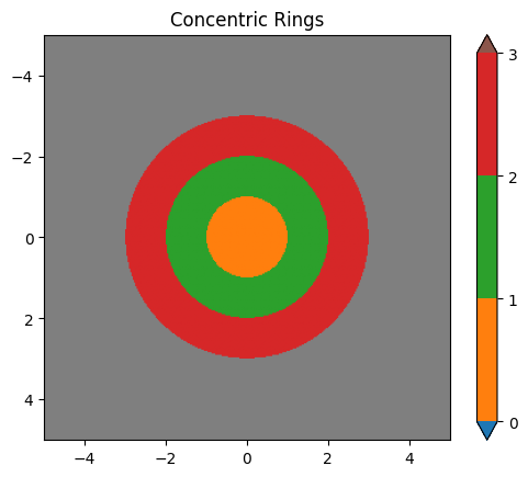
# Example 1: Concentric rings (geometric components)
visual_size = (10, 10)
ppd = 32

ring_stim = rings(visual_size=visual_size, ppd=ppd,
                  radii=(1, 2, 3),
                  intensity_rings=(0.2, 0.8, 0.4),
                  intensity_background=0.5)

plot_stim(ring_stim, mask="ring_mask", stim_name="Concentric Rings")
plt.show()

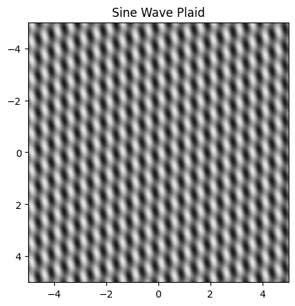
# Example 2: Sine wave plaid (complex composition)
grating1_params = {
    "visual_size": visual_size,
    "ppd": ppd,
    "frequency": 2,
    "intensities": (0.0, 1.0),
    "rotation": 0
}
grating2_params = {
    "visual_size": visual_size,
    "ppd": ppd,
    "frequency": 2,
    "intensities": (0.2, 0.8),
    "rotation": 45,
    "round_phase_width": False,
}

plaid_stim = plaid_sine(grating1_params, grating2_params)

plot_stim(plaid_stim, stim_name="Sine Wave Plaid")
plt.show()

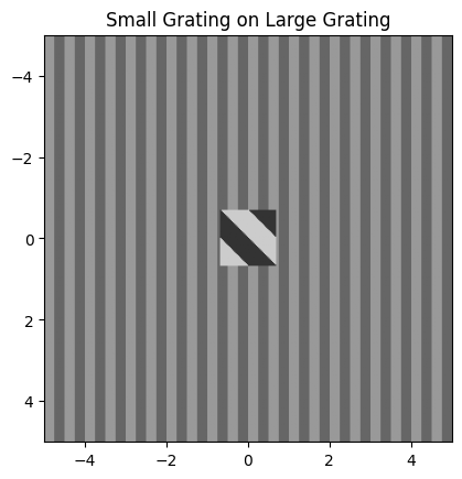
# Example 3: Small grating on larger grating (complete stimulus)
small_grating_params = {
    "ppd": ppd,
    "bar_width": 0.5,
    "n_bars": 4,
    "intensity_bars": (0.2, 0.8),
    "rotation": 45,
    "round_phase_width": False,
}

large_grating_params = {
    "visual_size": visual_size,
    "ppd": ppd,
    "frequency": 2,
    "intensity_bars": (0.4, 0.6),
    "rotation": 0
}

grating_stim = on_grating(small_grating_params=small_grating_params,
                         large_grating_params=large_grating_params)

plot_stim(grating_stim, stim_name="Small Grating on Large Grating")
plt.show()

/home/joris/Research/stimupy/stimupy/utils/resolution.py:350: UserWarning: Rounding shape; 4.296875 * 32.0 = 137.5 -> 137
  warnings.warn(f"Rounding shape; {visual_angle} * {ppd} = {fpix} -> {pix}")

Method 2: Simple array operations

When to use: For basic combinations where you want to apply operations across entire images.

Steps:

1. Create your component stimuli

2. Apply numpy operations (addition, subtraction, multiplication) to the "img" arrays

3. Wrap the result in a stimulus dictionary

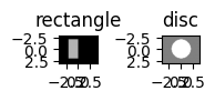
# Step 1: Create components
rectangle = shapes.rectangle(visual_size=(6,8), ppd=10,
                        rectangle_size=(4,2), rectangle_position=(1,2),
                        intensity_rectangle=.7)

disc = shapes.disc(visual_size=(6,8), ppd=10,
                        radius=2,
                        intensity_disc=1, intensity_background=.5)

plot_stimuli({"rectangle": rectangle, "disc": disc})
plt.show()

# Step 2: Apply operation
new_img = disc["img"] - rectangle["img"]

# Step 3: Create stimulus dictionary
composed_stim = {
    "img": new_img,
    "visual_size": disc["visual_size"],
    "ppd": disc["ppd"]
}

plt.imshow(new_img, cmap="gray")
plt.title("Simple subtraction")
plt.show()

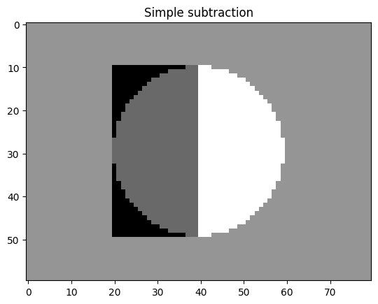
Limitation: This method operates on entire images, including background regions, which may not give you the precise control you need.

Method 3: Mask-based composition

When to use: When you need precise control over which regions are affected by operations.

Steps:

1. Create your component stimuli

2. Extract and combine the masks using logical operations

3. Use the combined mask to create your final image

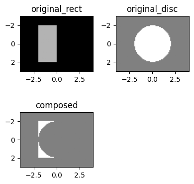
# Step 1: Create components (reusing from above)

# Step 2: Create logical mask combination
# Remove rectangle where it overlaps with disc
anti_join_mask = (rectangle["rectangle_mask"] == 1) & (~(disc["ring_mask"] == 1))

# Step 3: Create image using mask
composition = {
    "img": np.where(anti_join_mask, 1, .5),
    "anti_join_mask": anti_join_mask,
    "visual_size": disc["visual_size"],
    "ppd": disc["ppd"]
}

plot_stimuli({"original_rect": rectangle, "original_disc": disc, "composed": composition})

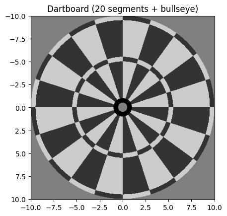
More complex example: Dartboard

from stimupy.stimuli.bullseyes import circular as bullseye_circular
from stimupy.stimuli.waves import square_angular

# Create dartboard by combining angular segments (pinwheel) and concentric rings
dartboard_size = (20, 20)
dartboard_ppd = 20

# Step 1: Create a bullseye stimulus (set of concentric rings)
bullseye = bullseye_circular(visual_size=dartboard_size, ppd=dartboard_ppd,
                    n_rings=20, intensity_background=0.5)

# Step 2: Create base dartboard (segments + bullseye)
# First set of angular segments
wheel1 = square_angular(visual_size=dartboard_size, ppd=dartboard_ppd,
                       n_segments=20, intensity_segments=(0.2, 0.8))

# Step 3: Combine segments with bullseye to create base dartboard
base_dartboard_img = wheel1["img"].copy()
base_dartboard_mask = wheel1["segment_mask"].copy()

# Add bullseye in center (override segments in center area)
bullseye_center = bullseye["ring_mask"] <= 2  # inner bullseye only
base_dartboard_img = np.where(bullseye_center, bullseye["img"], base_dartboard_img)
# Keep bullseye rings in mask
base_dartboard_mask = np.where(bullseye_center, bullseye["ring_mask"], base_dartboard_mask)

# Step 4: Create opposite segments for scoring rings
wheel2 = square_angular(visual_size=dartboard_size, ppd=dartboard_ppd,
                       n_segments=20, intensity_segments=(0.8, 0.2))  # reversed intensities

# Step 5: Replace selected scoring rings with opposite pattern
# Identify specific scoring rings (e.g., rings 11 and 20)
scoring_rings = (bullseye["ring_mask"] == 11) | (bullseye["ring_mask"] == 20)

# Final dartboard: base + scoring ring replacements
dartboard_img = base_dartboard_img.copy()
dartboard_img = np.where(scoring_rings, wheel2["img"], dartboard_img)

# Final mask: combine all regions
combined_mask = base_dartboard_mask.copy()
combined_mask = np.where(scoring_rings, bullseye["ring_mask"], combined_mask)

# Step 6: Create final dartboard stimulus
dartboard = {
    "img": dartboard_img,
    "mask": combined_mask,
    "visual_size": dartboard_size,
    "ppd": dartboard_ppd
}

plot_stim(dartboard, stim_name="Dartboard (20 segments + bullseye)")
plt.show()

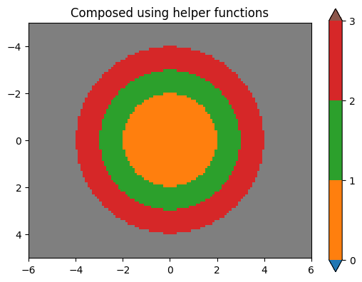
Using helper functions for mask-based composition

For standard mask-based workflows, stimupy provides helper functions that streamline the process:

Key functions:

• stimupy.components.combine_masks(): Merge multiple masks into one indexed mask

• stimupy.components.draw_regions(): Draw regions based on a mask with different intensities

from stimupy.components import combine_masks, draw_regions

# Step 1: Create multiple components
visual_size = (10, 12)
ppd = 10

disc = shapes.disc(visual_size=visual_size, ppd=ppd,
                   radius=2, intensity_disc=.5, intensity_background=.5)

ring_1 = shapes.ring(visual_size=visual_size, ppd=ppd,
                     radii=(2, 3), intensity_ring=1, intensity_background=.5)

ring_2 = shapes.ring(visual_size=visual_size, ppd=ppd,
                     radii=(3, 4), intensity_ring=0, intensity_background=.5)

# Step 2: Combine masks
combined_mask = combine_masks(disc["ring_mask"], ring_1["ring_mask"], ring_2["ring_mask"])

# Step 3: Draw regions with desired intensities
img = draw_regions(mask=combined_mask, 
                   intensities=[0.5, 1, 0],  # intensities for regions 1, 2, 3
                   intensity_background=0.5)

# Step 4: Create final stimulus
bullseye = {
    "img": img,
    "mask": combined_mask,
    "visual_size": visual_size,
    "ppd": ppd
}

plot_stim(bullseye, mask="mask", stim_name="Composed using helper functions")
plt.show()

Common mask operations:

• Intersection: (mask1 == 1) & (mask2 == 1)

• Union: (mask1 == 1) | (mask2 == 1)

• Difference: (mask1 == 1) & (~(mask2 == 1))

For more details on working with masks, see the Masks guide.

Choosing the right method

Method	Best for	Pros	Cons
Direct functions	Common patterns	Complete solution, optimized	Only for pre-defined patterns
Array operations	Simple combinations	Fast, straightforward	Limited control, affects entire image
Mask-based	Precise region control	Fine-grained control, helper functions available	More complex setup

General workflow

Regardless of method, the general composition workflow is:

1. Plan your composition: Identify the components and how they should interact

2. Create components: Generate the basic geometric elements

3. Combine appropriately: Choose the method that best fits your needs

4. Validate result: Check that the composition matches your intention

The stimupy.components provide the building blocks, and these composition methods let you combine them into more complex visual stimuli.